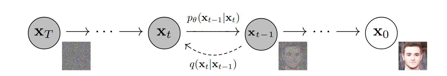
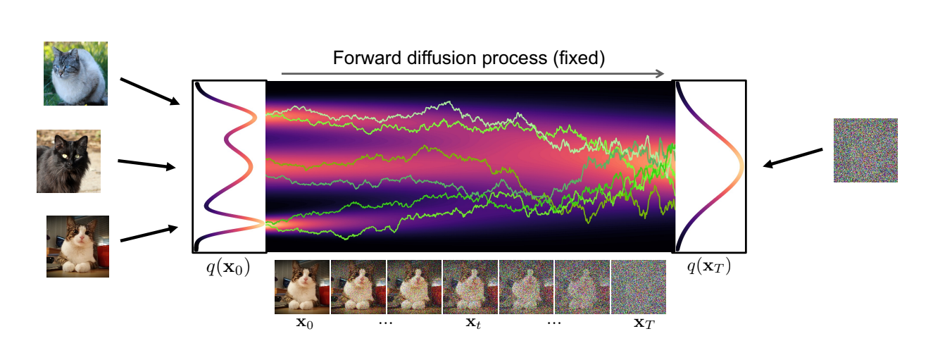
(Fixed) Forward diffusion process that gradually adds noise to input
(Learnt / Generative) Reverse denoising process that learns to generate data by denoising
The goal of a diffusion model is to learn the reverse denoising process to iteratively undo the forward process
In this way, the reverse process appears as if it is generating new data from random noise!
Assumptions:
Ancestral sampling: data distribution can be represented as a series of increasingly noisy versions, with the original data being the "clean" version. This allows them to learn the process of progressively denoising the data.
Gaussian noise: The noise added during the forward diffusion is generally assumed to be Gaussian, with a mean of 0 and a gradually increasing variance
Markov property: forward diffusion process is assumed to follow a Markov property, meaning the transition probability at any step depends only on the previous step and not on the entire history.
Forward Process / diffusion process
Goal
Gradually adds Gaussian noise to the data by Markov Chain
Markov chain or Markov process is a stochastic process describing a sequence of possible events in which the probability of each event depends only on the state attained in the previous event. The distribution at a particular time step only depends on the sample from the immediate previous step
Why Markov Chain can be used?
The forward process is designed such that each image xt is generated by adding a small amount of noise to the previous image xt−1. In other words, xt∼q(xt∣xt−1), meaning that this process only depends on the immediately preceding state and not on any earlier states. This fully aligns with the definition of a Markov chain: “the distribution of the current state depends only on the previous state.” Therefore, it is appropriate to model this process as a Markov chain, since the forward diffusion is inherently a locally dependent stochastic process—by design, it is Markovian.
Why using Markov Chain?
Simplified modeling and mathematical derivation: Instead of modeling complex global noise all at once, the problem is broken down into a sequence of small incremental changes. Each step only needs to learn how to “add a small amount of noise,” making the modeling and training process more tractable. Mathematically, this also facilitates the derivation of a complete probabilistic model, enabling the use of tools such as KL divergence for optimization.
Facilitates the derivation and sampling of the reverse process: The denoising process can be constructed step by step in reverse, with each step theoretically grounded. At each stage, the denoising prediction only needs to rely on the current noisy state, without requiring knowledge of the full noise trajectory.
Why using Gaussian noise?
The Gaussian distribution is the most fundamental, simple, and controllable distribution among continuous probability distributions. If Gaussian noise is continuously added to an image, the distribution of the image will eventually converge to the standard normal distribution N(0,I). This gives the forward process a clear and simple “endpoint.” In other words, using Gaussian noise allows us to know exactly what the process will converge to—pure noise—and this final distribution is easy to sample from.
The sum of Gaussian noises is still Gaussian, which makes mathematical derivations more tractable. Since the process remains a composition of Gaussian distributions over multiple steps, we can directly derive the probability distribution between any two time steps—for example, the distribution of noise at step 100 given the original image.
Gaussian noise is highly compatible with the denoising task: In image processing, “Gaussian denoising” is a well-established problem, and many models have been developed to handle it. Therefore, training a model to predict how to recover an image from Gaussian noise is both practically feasible and relatively easy to converge.
The Gaussian distribution is differentiable and has closed-form expressions: For tasks such as taking derivatives, performing maximum likelihood estimation, and optimizing loss functions, the Gaussian distribution is highly convenient. Its probability density function (PDF) and KL divergence have analytical closed-form solutions, making computation efficient and stable.
Get approximate posterior q(x1:T∣x0)
q(x1:T∣x0):=t=1∏Tq(xt∣xt−1)
Given x0, the probability of generate the sequence x1:T={x1,x2,…,xT}
According to Markov Chain and the chain rule of probability
Each transition is parameterised as a diagonal Gaussian
diagonal Gaussian
Each dimension is independent (since the covariances are zero);
Each dimension has its own variance σi2;
There is no linear correlation between different dimensions.
Why diagonal Gaussian
Simplified computation: The covariance matrix is diagonal, making sampling and likelihood calculation easier.
High computational efficiency: No need to store or manipulate complex matrices.
Sufficient flexibility: For many tasks, the independence assumption is enough to generate high-quality samples.
More stable training.
By adding Gaussian noise, the transition probability at each step, q(xt∣xt−1) can be defined as a conditional Gaussian distribution.
Variance (schedule): β1,...,βt
βt are hyperparameters, follows a fix schedule
noise schedule: how much noise you are adding at each step
variane matrix: βtI (Assume the noise is isotropic, i.e., it has the same variance in every dimension.)
β increase with time: β1<β2<...<βt
{βt∈(0,1)}t=1T → 1−βt∈(0,1) → mean of each of Gaussian close to 0
Mean: 1−βtxt−1
Use the data from the previous step as the basis for scaling.
mean of each of Gaussian close to 0
T : timestep
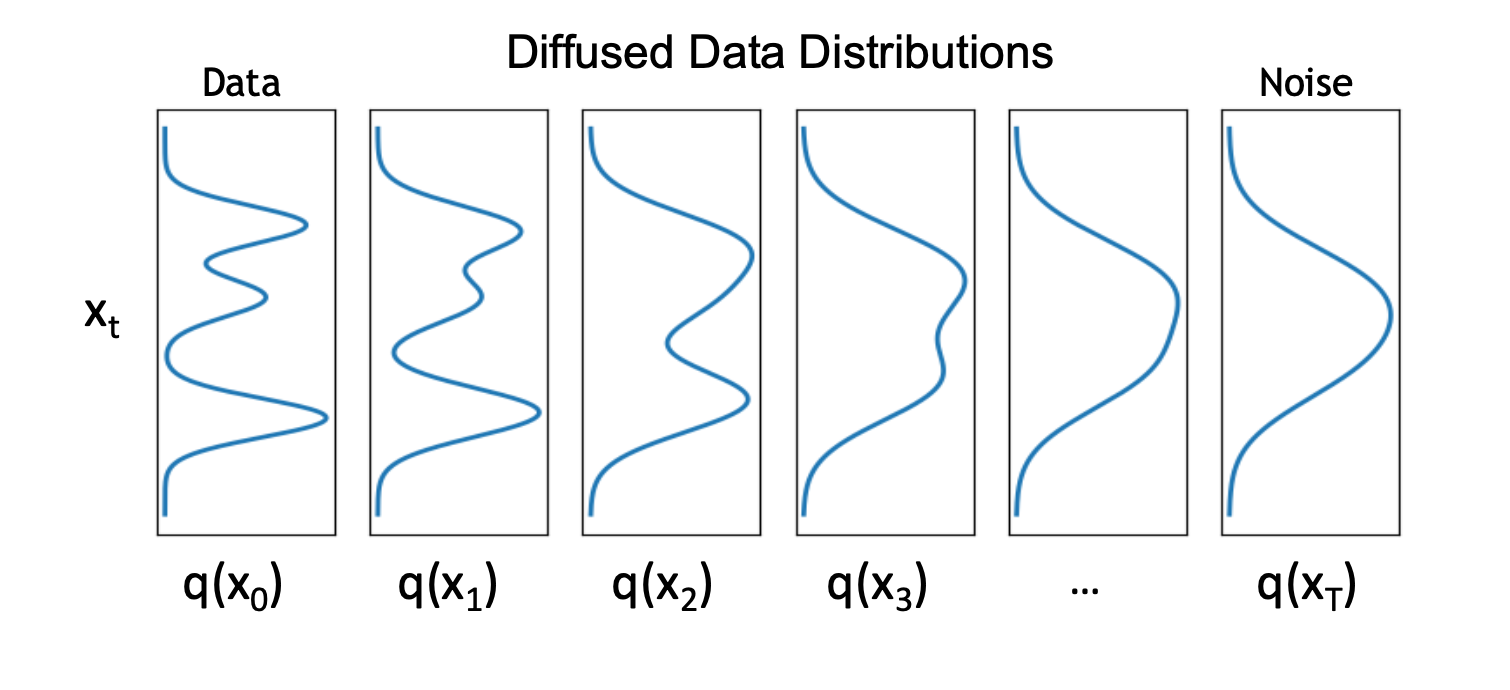
T→∞limq(xT∣x0)=N(0,I)
In practical, T is thousands, T set to be large → set βt to be very small
Why small βt ? so the reverse won't be too difficult
As time step increases, the more feature of original inputs were destroyed
T→∞, pure random noise, isotropic gaussian q(xT∣x0)=N(0,I)
Tricks for efficient training
Trick is basically showing that you can directly express xt in terms of x0, which means you can directly go from initial image to a noisy version at given timestep → simplify all the math
the form of q(xt∣x0) can be recursively derived through repeated applications of the reparameterization trick.
Suppose that we have access to 2T random noise variables {ϵ∗,ϵt}t=0T {t∗, t}tT=0 iid ∼ N (; 0, I). Then, for an arbitrary sample xt∼q(xt∣x0), we can rewrite it as:
make a image with pure noise and denoise until back to the original image
learn the reverse denoising process to iteratively undo the forward process
The reverse process appears as if it generating new data from random noise
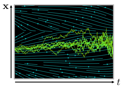
Diffused Data Distribution q(xt)
In generation, we follow:
Sample xT∼N(xT;0,I)
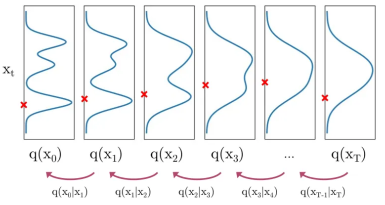
Iteratively sample xt−1∼q(xt−1∣xt)
q(xt−1∣xt) is unknown
distribution of xt−1 conditioned on xt is hard to find cuz some terms in the math is hard/intractable to compute because you have to know what the distribution is like exactly
Approximate the reverse process / learn to calculate the q(xt−1∣xt)
Several ways to try:
math equation
plot the 5 examples
For small enough forward steps, the reverse process step q(xt−1∣xt) can be estimated as Gaussian Distribution too (derived from stochastic differential equation), therefore we have:
This gaussian(defined by mean and variance) learn from NN
Optimisation
ELBO: Evidence Lower Bound
Objective: recover the likelihood of purely our observed data p(x)
Method 1
obtain distribution of observed data x by explicitly marginalize out the latent variable z
p(x)=∫p(x,z)dz
Directly computing and maximizing the likelihood p(x) is difficult because it involves integrating out all latent variables z in Equation, which is intractable for complex models.
logp(x)=log∫p(x,z)dz=log∫qϕ(z∣x)p(x,z)qϕ(z∣x)dz=logEqϕ(z∣x)[qϕ(z∣x)p(x,z)]≥Eqϕ(z∣x)[logqϕ(z∣x)p(x,z)](Apply Equation 1)(Multiply by 1 = qϕ(z∣x)qϕ(z∣x))(Definition of Expectation)(Apply Jensen’s Inequality)
However, this does not supply us much useful information about what is actually going on underneath the hood; crucially,
this proof gives no intuition on exactly why the ELBO is actually a lower bound of the evidence, as Jensen’s Inequality handwaves it away.
simply knowing that the ELBO is truly a lower bound of the data does not really tell us why we want to maximize it as an objective. i.e. why optimizing the ELBO is an appropriate objective at all.
Method 2
obtain distribution of observed data x by chain rule of probability
p(x)=p(z∣x)p(x,z)
Directly computing and maximizing the likelihood p(x) is difficult because it involves having access to a ground truth latent encoder p(z∣x) in Equation.
better understand the relationship between the evidence and the ELBO
logp(x)=logp(x)∫qϕ(z∣x)dz=∫qϕ(z∣x)(logp(x))dz=Eqϕ(z∣x)[logp(x)]=Eqϕ(z∣x)[logp(z∣x)p(x,z)]=Eqϕ(z∣x)[logp(z∣x)qϕ(z∣x)p(x,z)qϕ(z∣x)]=Eqϕ(z∣x)[logqϕ(z∣x)p(x,z)]+Eqϕ(z∣x)[logp(z∣x)qϕ(z∣x)]=Eqϕ(z∣x)[logqϕ(z∣x)p(x,z)]+DKL(qϕ(z∣x)∥p(z∣x))≥Eqϕ(z∣x)[logqϕ(z∣x)p(x,z)](Multiply by 1 = ∫qϕ(z∣x)dz)(Bring evidence into integral)(Definition of Expectation)(Apply Equation 2)(Multiply by 1 = qϕ(z∣x)qϕ(z∣x))(Split the Expectation)(Definition of KL Divergence)(KL Divergence always ≥0)
evidence is equal to the ELBO plus the KL Divergence (which is non-negative) between the approximate posterior qϕ(z∣x) and the true posterior p(z∣x). → the value of the ELBO can never exceed the evidence.
why we seek to maximize the ELBO
want to optimize the parameters of our variational posterior qφ(z|x) to exactly match the true posterior distribution qϕ(z∣x) , which is achieved by minimizing their KL Divergence (ideally to zero). Unfortunately, it is intractable to minimize this KL Divergence term directly, as we do not have access to the ground truth p(z∣x) distribution.
notice that on the left hand side of Equation 15, the likelihood of our data (and therefore our evidence term p(x)) is always a constant with respect to ϕ, as it is computed by marginalizing out all latents x from the joint distribution p(x,z) and does not depend on ϕ whatsoever.
Since the ELBO and KL Divergence terms sum up to a constant, any maximization of the ELBO term with respect to ϕ necessarily invokes an equal minimization of the KL Divergence term. Thus, the ELBO can be maximized as a proxy for learning how to perfectly model the true latent posterior distribution; the more we optimize the ELBO, the closer our approximate posterior gets to the true posterior.
Additionally, once trained, the ELBO can be used to estimate the likelihood of observed or generated data as well, since it is learned to approximate the model evidence log p(x).
qϕ(z∣x)
is a flexible approximate variational distribution with parameters ϕ that we seek to optimize.
can be thought of as a parameterizable model that is learned to estimate the true distribution over latent variables for given observations x
it seeks to approximate true posterior p(z∣x)
ELBO=Eqϕ(z∣x)[logqϕ(z∣x)p(x,z)]
increase the lower bound by tuning the parameters ϕ to maximize the ELBO, we gain access to components that can be used to model the true data distribution and sample from it, thus learning a generative model.
ELBO becomes a proxy objective with which to optimize a latent variable model;
Variational Autoencoders
Eqϕ(z∣x)[logqϕ(z∣x)p(x,z)]=Eqϕ(z∣x)[logqϕ(z∣x)pθ(x∣z)p(z)]=Eqϕ(z∣x)[logpθ(x∣z)]+Eqϕ(z∣x)[logqϕ(z∣x)p(z)]=Eqϕ(z∣x)[logpθ(x∣z)]−DKL(qϕ(z∣x)∥p(z))=reconstruction termEqϕ(z∣x)[logpθ(x∣z)]−prior matching termDKL(qϕ(z∣x)∥p(z))(Chain Rule of Probability)(Split the Expectation)(Definition of KL Divergence)
Encoder qϕ(z∣x): transforms inputs into a distribution over possible latents
Decoderpθ(x∣z): a deterministic function that convert a given latent vector z into an observation x
Reconstruction Term
this ensures that the learned distribution is modeling effective latents that the original data can be regenerated from
Prior matching term
measures how similar the learned variational distribution is to a prior belief held over latent variables.
Minimizing this term encourages the encoder to actually learn a distribution rather than collapse into a Dirac delta function.
** Maximizing the ELBO is thus equivalent to maximizing its first term and minimizing its second term.
ELBO optimized jointly over parameters ϕ and θ in VAE
The VAE utilizes the reparameterization trick and Monte Carlo estimates to optimize the ELBO jointly over ϕ and θ.
Monte Carlo estimates
The encoder of the VAE is commonly chosen to model a multivariate Gaussian with diagonal covariance, and the prior is often selected to be a standard multivariate Gaussian
the KL divergence term of the ELBO can be computed analytically
the reconstruction term can be approximated using a Monte Carlo estimate.
reparameterization trick
x∼N(μ,σ2)→x=μ+σϵwithϵ∼N(ϵ;0,I)
Why use reparameterizarion trick
each z(l) that our loss is computed on is generated by a stochastic sampling procedure, which is generally non-differentiable.
what is reparameterization trick
rewrites a random variable as a deterministic function of a noise variable;
allows for the optimization of the non-stochastic terms through gradient descent.
arbitrary Gaussian distributions can be interpreted as standard Gaussians (of which is a sample) that have their mean shifted from zero to the target mean μ by addition, and their variance stretched by the target variance σ2
by the reparameterization trick, sampling from an arbitrary Gaussian distribution can be performed by sampling from a standard Gaussian, scaling the result by the target standard deviation, and shifting it by the target mean.
use reparameterization trick in ELBO of VAE
z=μϕ(x)+σϕ(x)⊙ϵwithϵ∼N(ϵ;0,I)
represents an element-wise product
Under this reparameterized version of z, gradients can then be computed with respect to ϕ as desired, to optimize μϕ and σϕ.
Variational Autoencoders are particularly interesting when the dimensionality of z is less than that of input x, as we might then be learning compact, useful representations.
Furthermore, when a semantically meaningful latent space is learned, latent vectors can be edited before being passed to the decoder to more precisely control the data generated.
The easiest way to think of a Variational Diffusion Model (VDM) is simply as a MHVAE with three key restrictions:
The latent dimension is exactly equal to the data dimension → represent both true data samples and latent variables as xt
The structure of the latent encoder at each timestep is not learned; it is pre-defined as a linear Gaussian model. In other words, it is a Gaussian distribution centered around the output of the previous timestep.
The Gaussian parameters of the latent encoders vary over time in such a way that the distribution of the latent at final timestep T is a standard Gaussian.
ELBO in Variational Diffusion Model
logp(x)=log∫p(x0:T)dx1:T=log∫q(x1:T∣x0)p(x0:T)q(x1:T∣x0)dx1:T=logEq(x1:T∣x0)[q(x1:T∣x0)p(x0:T)]≥Eq(x1:T∣x0)[logq(x1:T∣x0)p(x0:T)]=Eq(x1:T∣x0)[log∏t=1Tq(xt∣xt−1)p(xT)∏t=1Tpθ(xt−1∣xt)]=Eq(x1:T∣x0)[logq(xT∣xT−1)∏t=1T−1q(xt∣xt−1)p(xT)pθ(x0∣x1)∏t=2Tpθ(xt−1∣xt)]=Eq(x1:T∣x0)[logq(xT∣xT−1)∏t=1T−1q(xt∣xt−1)p(xT)pθ(x0∣x1)∏t=1T−1pθ(xt∣xt+1)]=Eq(x1:T∣x0)[logq(xT∣xT−1)p(xT)pθ(x0∣x1)]+Eq(x1:T∣x0)[logt=1∏T−1q(xt∣xt−1)pθ(xt∣xt+1)]=Eq(x1:T∣x0)[logpθ(x0∣x1)]+Eq(x1:T∣x0)[logq(xT∣xT−1)p(xT)]+Eq(x1:T∣x0)[t=1∑T−1logq(xt∣xt−1)pθ(xt∣xt+1)]=Eq(x1:T∣x0)[logpθ(x0∣x1)]+Eq(x1:T∣x0)[logq(xT∣xT−1)p(xT)]+t=1∑T−1Eq(x1:T∣x0)[logq(xt∣xt−1)pθ(xt∣xt+1)]=Eq(x1∣x0)[logpθ(x0∣x1)]+Eq(xT−1,xT∣x0)[logq(xT∣xT−1)p(xT)]+t=1∑T−1Eq(xt−1,xt,xt+1∣x0)[logq(xt∣xt−1)pθ(xt∣xt+1)]=reconstruction term Eq(x1∣x0)[logpθ(x0∣x1)]−prior matching term Eq(xT−1∣x0)[DKL(q(xT∣xT−1)∥p(xT))]−t=1∑T−1consistency term Eq(xt−1,xt+1∣x0)[DKL(q(xt∣xt−1)∥pθ(xt∣xt+1))]
reconstruction term
prior matching term:
minimized when the final latent distribution matched the Gaussian prior.
This term requires no optimization
as we assume the large enough T, such that final distribution is Gaussian, this term turns zero immediately
consistency term
minimized when we train pθ(xt∣xt+1) to match the Gaussian distribution q(xt∣xt−1)
Approximate ELBO with lower variance
From previous equations, all terms of ELBO are calculated as expectations, therefore can be approximated by Monte Carlo estimates.
However, actually optimizing the ELBO using the terms we just derived might be suboptimal; because the consistency term is computed as an expectation over two random variables{xt−1,xt+1} for every timestep, the variance of its Monte Carlo estimate could potentially be higher than a term that is estimated using only one random variable per timestep.
Thus try yo derive an expectation over only one random variable.
Thus, the xt−1∼q(xt−1∣xt,x0) is normally distributed, with mean μq(xt,x0) that is a function of xt and x0, and variance Σq(t) as a function of α coefficients
pθ(xt−1∣xt)
From above, the ground truth q(xt−1∣xt,x0) follows the normal distribution. Thus, we also model pθ(xt−1∣xt) as a Gaussian
the variance can be computed since all variance terms are known to be frozen at each timestep and can set the variances of the two Gaussians to match exactly
must parameterise its mean as a function of xt
Denoising matching term
recall the KL divergence definition, we want to optimize a μθ(xt,t) to match μq(xt,x0)
Therefore, optimizing a diffusion model boils down to learning a neural network to predict the original ground truth image from arbitrarily noisified version of it.
Furthermore, minimizing the summation term of our derived ELBO objective across all noise levels can be approximated by minimizing the expectation over all timesteps, which can then be optimized using stochastic samples over timesteps.
Here, ϵ^θ(xt,t) is a neural network that learns to predict the source noise ϵ0∼N(0,I) that determines xt from x0.
We have therefore shown that learning a VDM by predicting the original image x0 is equivalent to learning to predict the noise; empirically, however, some works have found that predicting the noise resulted in better performance.
So you are trying to predict the noise that was added at time 0 to get to the time t. Know how to add then know how to subtract
Interpretation 2: Score function
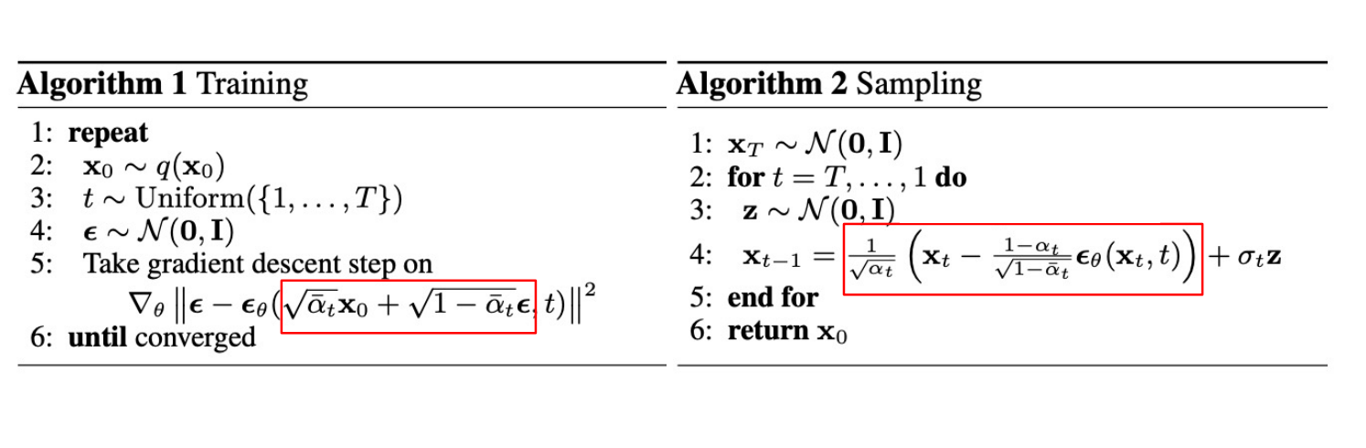
Training
Load in some images from the training data
Add noise, in different amounts.
Remember, we want the model to do a good job estimating how to ‘fix’ (denoise) both extremely noisy images and images that are close to perfect.
Feed the noisy versions of the inputs into the model
Evaluate how well the model does at denoising these inputs
Use this information to update the model weights
pass that noised image into your model, and predict the noise added
minimise the predict noise with the actual noise
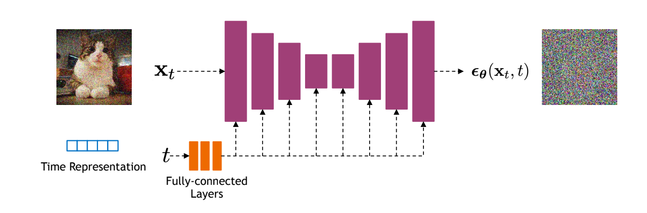
Training Architecture
Diffusion models often use U-Net architectures with ResNet blocks and self-attention layers to represent ϵ^θ(xt,t)
Time representation: sinusoidal positional embeddings or random Fourier features.
Time features are fed to the residual blocks using either simple spatial addition or using adaptive group normalization layers.
Parameters
βt and σt2 control the variance of the forward diffusion and reverse denoising processes respectively.
Often a linear schedule is used for βt, and σt2 is set equal to βt .
Kingma et al. NeurIPS 2022 introduce a new parameterization of diffusion models using signal-to-noise ratio (SNR), and show how to learn the noise schedule by minimizing the variance of the training objective.
We can also train σt2 while training the diffusion model by minimizing the variational bound (Improved DPM by Nichol and Dhariwal ICML 2021) or after training the diffusion model (Analytic-DPM by Bao et al. ICLR 2022).
Generation
start from image of random noise
pass this completely random noise into the model
model predict some noise from that
subtract the predicted noise from the noise image
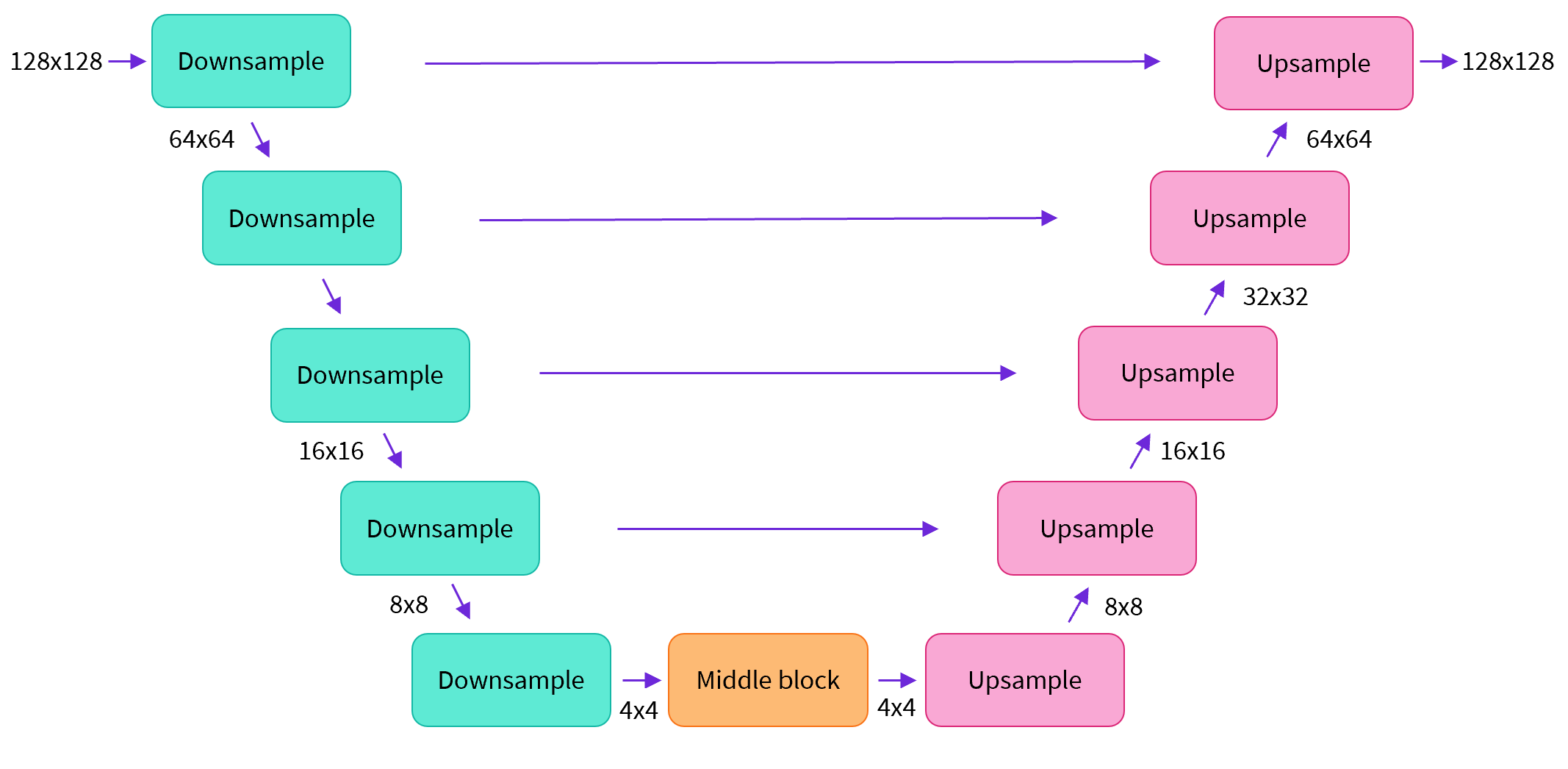
UNet
A key feature of this model is that it predicts images of the same size as the input, which is exactly what we need here.
When dealing with higher-resolution inputs you may want to use more down and up-blocks, and keep the attention layers only at the lowest resolution (bottom) layers to reduce memory usage.
Encoder Downsampling
The encoder is responsible for feature extraction and representation learning. It uses specific computational methods to represent the entire image with a more compact form of data. This smaller representation captures high-level characteristics of the image, rather than fine-grained pixel-level details. The more compact the data, the more abstract and semantic the representation becomes, which helps in understanding the overall content of the image.
For example, consider an image of a cat playing in front of a house. The original image retains all fine details, but to identify the presence of the cat and the house, a model would need to perform extensive operations across all pixels. In contrast, when downsampled to a coarser representation, these high-level objects like “cat” and “house” become easier to recognize.
The encoder module can be implemented using top-tier feature extractors such as ResNet, VGG, or EfficientNet, which gives it strong potential for both engineering applications and research advancements.
At the same time, the encoder can improve robustness to noisy perturbations, reduce the risk of overfitting, lower computational cost, and enlarge the receptive field, among other benefits.
Decoder Upsampling
The decoder is responsible for restoring the macro-level, low-resolution representation of an image back to its original resolution.
For example, in image segmentation (where the goal is to separate objects from the background), we may identify object boundaries and key features in the downsampled high-level representation, but this information must ultimately be mapped back to the original image size to be useful.
But naturally, one might ask: after so much downsampling and loss of detail, how can we possibly recover fine-grained information during upsampling? This is where skip connections come into play.
The decoder reconstructs the feature map to its original resolution, and through skip connections, it fuses shallow-layer spatial information with deep-layer semantic understanding. Like the encoder, the decoder can also be implemented using powerful models such as ResNet, VGG, or EfficientNet, making U-Net variants highly diverse and adaptable—offering strong potential for architectural innovation.
Additionally, the decoder has inherent denoising capabilities, helping to refine outputs by integrating coarse-to-fine representations and filtering out irrelevant noise from the final result.
Skip connection
At each upsampling layer, the decoder concatenates the corresponding feature maps from the encoder (i.e., from the same resolution level on the left) and uses this combined information as input for the next upsampling stage.
The reason for doing this is intuitive:
Each layer in the encoder preserves image details to varying degrees, while the decoder layers—obtained through upsampling—primarily carry high-level, abstract information but lack fine-grained details.
By concatenating the encoder’s detailed feature maps with the decoder’s abstract representations, the network gains access to both macro-level semantics and micro-level details.
As a result, every layer in the decoder has a multi-scale understanding of the image, making it capable of performing various tasks such as image segmentation and semantic image generation.
Then we need to get the score function ∇xtlogqt(xt)
Naïve idea, learn model for the score function by direct regression? But ∇xtlogqt(xt) (score of the marginal diffused density qt(xt) is not tractable!
θmindiffusiontEt∼U(0,T)diffused data xtExt∼qt(xt)neural networksθ(xt,t)−score ofdiffused data (marginal)∇xtlogqt(xt)22
Instead, diffuse individual data points x0. Diffused qt(xt∣x0)is tractable!
θmindiffusiontEt∼U(0,T)data sample x0Ex0∼q0(x0)diffused data sample xtExt∼qt(xt∣x0)neural networksθ(xt,t)−score of diffuseddata sample∇xtlogqt(xt∣x0)22
Specifically, we can do the Denoising Score Matching
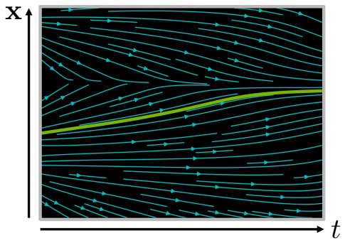
The vector field between noise and data distribution can be learnt directly via Flow Matching.
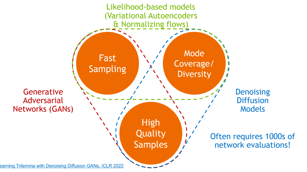
What makes a good generative model?
Model Improvements
Algorithmic Improvements
Learned variance
Deterministic Sampler
DDPM
DDIM
Score-based Models
Faster Sampling
DDIM
EDM
SGM
PFGM
Architecture Improvements
Classifier Guidance
Key idea: add an additional term in the sampling process to direct towards the desired class
Train a classifier on noisy images
use gradient to guide towards a class label
Results: similar image quality but better diversity
Classifier-Free Diffusion Guidance
Motivation: Classifier Guidance enabled “low temperature” / “sharper” samples, but we want to achieve this without additional classifier to train, purely in the generative model itself
Key idea: consider extra term in classifier free guidance sampling + apply Bates rules